Summary:
· Understanding the determinants of savings is fundamental to many economic issues (smoothing consumption over time, investment, monetary policy decisions, etc.);
· Technological advances are helping us to better understand these determinants by linking theory and empirical observations;
· This article highlights some of the progress made in this area and how it can be useful in economic policy.


Savings are a fundamental economic variable and affect macroeconomic dynamics in both the short and long term. The response of savings to interest rates, for example, influences the effectiveness of monetary policy. In the long term, savings determine investment and therefore the level of capital per capita. Even today, economists are still trying to understand which factors have the greatest effect on savings (and therefore on consumption). For a long time, research was limited by technical constraints in combining theory and data: research based on the life cycle model (see below) initially focused on testing the theory without any major practical applications.
Now, technical advances have made it possible to make the model much more realistic, to compare it with data, and to use it to assess the impact of various policies or phenomena on major economic issues. This article aims to briefly report on this development, to show the progress it has enabled, and to describe some of its limitations.
From theory to data
The standard model used to represent household savings behavior is the life cycle model developed by Modigliani and Brumberg (1954). In its simplest form, households save for retirement because they want to smooth their consumption over time: anticipating lower income in retirement, they save so that their consumption during retirement will be close to that during their working life.
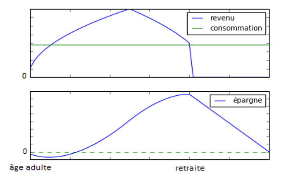
Figure 1 presents a very simple version of this model in which households want to maintain the same level of consumption over time. We assume that they know exactly how their income will evolve in advance and that there is no uncertainty. Income is represented by the blue curve in the upper panel. It increases after adulthood, then decreases after a certain age, and finally equals zero at retirement (in the absence of a pension plan[3]). We can see that in the early years, the household consumes more than its income because its income is relatively low. To do this, it borrows, as shown in the lower panel where savings are negative. At a certain point, income exceeds consumption and savings increase. Here, savings increase until retirement. Once retirement age is reached, income is zero and consumption is financed by the dis-accumulation of savings. We can see that savings decrease after retirement age.
Figure 1: Simplified version of the life cycle model
For a long time, research based on this theory was limited to testing the theory’s limited predictions because, as soon as the risks faced by households (unemployment, illness, etc.) are introduced to make the model more realistic, it cannot be solved analytically. Of course, it can be argued that savings can be studied without a strict theoretical framework, and many important studies are based on reduced-form methods. However, when studying savings, it becomes difficult to examine certain issues without a more rigorous framework. To give an example, studying the savings behavior of retired households is particularly complex due to a strong selection bias because, over time, the wealthiest households (i.e., those with the greatest capacity to save) become overrepresented due to lower mortality than poorer households (see De Nardi, French, Jones (2010)). In general, for certain issues, the risks faced by different population groups require a structural approach (i.e., an approach where behaviors are represented through a model).
Currently, advances in numerical resolution make it possible to simulate consumption and saving behaviors predicted by life cycle models that are much richer than the initial model, where risks and public policies can be modeled realistically. In addition, these models can now be estimated, making it possible to verify whether the model is capable of quantitatively reproducing empirical facts and whether the structural parameters of the model are correctly identified. We are therefore able to reject the model if it cannot reproduce certain important empirical facts. These models can also take into account different types of heterogeneity, whether in terms of risks (e.g., the risk of unemployment differs according to education) or preferences[5], and thus take into account the inequalities observed. One advantage of these models is that risks can be explicitly modeled in the model, which avoids many biases. Finally, this development has made it possible to identify the factors that could mainly explain the savings behaviors (and in some cases insurance, retirement age, etc.) observed in the data.
From a rejection of standard theory to models where constraints and risks predominate
In general, older research has tested Euler’s equation[6], which is a condition of equilibrium in the life cycle model. These tests have generally led to a rejection of the model in its standard version, which has been confirmed by recent research. Indeed, in its simple version, the model has difficulty explaining many empirical facts, such as the increase in consumption inequalities over time, or even the general pattern of consumption according to age that can be observed in the data. For example, consumption is very close to income among young households (aged 25-35), whereas according to standard life cycle theory, given that income tends to increase with age, these households should consume more than their income through borrowing (bank loans, mortgages, etc.). This phenomenon can be explained by the presence of credit constraints, but also by the presence of risks on future income[7] (see Gourinchas and Parker (2002)).
Furthermore, particularly in the United States, we observe that retired households tend not to draw down their savings[8], or if they do, only to a small extent. However, according to standard life cycle theory, households accumulate wealth in the form of assets during their working lives and draw down this wealth during retirement. Two explanations currently appear plausible to explain this phenomenon:
- De Nardi, French, and Jones (2010) show, for example, that the low level of dissaving among retired households in the United States (over the period 1996-2006) can be explained by the presence of healthcare expenses (particularly those related to dependency), which can be very high in old age. Their model accurately reproduces the wealth dynamics of retired American households using plausible behavioral parameters[9]. As mentioned above, one of the advantages of this type of model is that mortality bias can be corrected by introducing it directly into the model.
- Another explanation is the presence of significant bequest motives, i.e., a strong preference among individuals to leave an inheritance. This is demonstrated in particular by Ameriks et al. (2010) and Lockwood (2016). In particular, Lockwood (2016) shows that a model in which bequest motives are significant, in addition to the precautionary motive to cover healthcare expenses, can explain both the low level of household savings and the low demand for long-term care insurance. De Nardi, French, and Jones (2016) show that significant bequest motives also help to reproduce the proportion of retirees using Medicaid[10].
Using behavioral models to assess the effect of policies
One of the advantages of the models described above is that they are behavioral models, i.e., they attempt to replicate how individuals react endogenously to a given environment. They can therefore be used to simulate the effect of different policies, for example in terms of well-being or distribution. De Nardi, French, and Jones (2016), for example, use their model to assess the effect of improved Medicaid coverage in terms of welfare. An extension of Medicaid increases the share of consumption that is insured (and thus reduces the need to maintain precautionary savings), but also increases the level of taxes. There is therefore a trade-off. They show that the value in terms of well-being for individuals of having access to Medicaid is greater than its cost, but that an extension of Medicaid would have a benefit in terms of well-being that would be lower than its cost. They therefore conclude that the size of Medicaid seems appropriate. Of course, distributional and equality considerations can also be taken into account when assessing whether the program should be expanded, and this model can accommodate such an analysis.
To illustrate with another example, Low and Pistaferri (2015) use a life cycle model to study whether expanding the disability insurance program in the United States would be beneficial overall. This program insures people who are unable to work due to their health condition, but it can also lead to moral hazard, where people who are able to continue working try to take advantage of it. Using their model, Low and Pistafferi (2015) show that expanding the program would have a beneficial effect because the increase in well-being due to better insurance more than offsets the negative effect of moral hazard.
This type of model can also be used to study issues at the macroeconomic level. For example, Wong (2016) studies the elasticity of consumption to interest rates for different categories and ages, and shows the mechanisms that explain these differences. She uses her model to show that the elasticity of aggregate consumption to interest rates can decrease sharply when the average age is higher, thereby reducing the transmission of monetary policy to consumption.
What are the limitations?
The few examples above show that progress has been made in understanding the determinants of savings behavior and how it interacts with other dimensions (insurance, labor market participation, etc.). Nevertheless, certain limitations remain:
- First, even though the models used are very rich, they can only take into account a limited number of variables due to current computational limitations. One advantage, however, is that this limitation forces researchers to be parsimonious, thus avoiding overly complex models and keeping them intelligible and intuitive.
- Second, these models have so far done relatively little to incorporate behavioral biases or take into account differences in individuals’ beliefs. The (difficult) question is which biases or beliefs are quantitatively important and which are not.
- Finally, the conclusions obtained with this type of model depend on the model itself. It can be shown that a certain model is consistent with certain empirical observations, but the question remains as to whether another model, based on other assumptions, could not do the same. This observation calls into question existing results when other alternatives are plausible.
Despite these limitations, the progress made in this research is undeniable and provides a better understanding of the important issue of the determinants of savings.
Conclusion
In conclusion, we have seen that research seeking to better understand the determinants of savings has made major progress in recent years, opening up the possibility of better understanding the effect of certain economic policies, such as reforms and monetary policy. This development has been made possible by advances in numerical resolution, which allow theoretical models to be compared with empirical observations.
References
Ameriks J., Caplin A., Laufer S., and Van Nieuwerburgh S., » The Joy of Giving or Assisted Living? Using Strategic Surveys to Separate Public Care Aversion from Bequest Motives , » The Journal of Finance, 2011
Attanasio O. and Weber G. « Consumption and Saving: Models of Intertemporal Allocation and Their Implications for Public Policy,« Journal of Economic Literature, Vol. 48, No. 3, pp. 693-751, Sept. 2010
De Nardi M., French E., and Jones J., » Why Do the Elderly Save? The Role of Medical Expenses, » Journal of Political Economy Vol. 118, No. 1 (February 2010), pp. 39-75
Gourichas P.O. and Parker J. « Consumption over the Life Cycle, » Econometrica, Vol. 70, No. 1 pp. 47-89, Jan. 2002
Lockwood L. « Incidental Bequests: Bequest Motives and the Choice to Self-Insure Late-Life Risks, » 2016
Low H. and Pistaferri L. » Disability Insurance and the Dynamics of the Incentive Insurance Trade-Off, » The American Economic Review, 2015
Modigliani F. and Brumberg R. « Utility Analysis and the Consumption Function: An Interpretation of Consumption Data, » Post-Keynesian Economics, pp. 388-436, New Brunswick: Rutgers University Press, 1954.
Wong A. » Population Aging and the Transmission of Monetary Policy to Consumption , » 2016
For those who want to learn more, see, for example, Mariacristina De Nardi’s presentation: https://www.youtube.com/watch?v=keGlwPrcJ4c&feature=youtu.be
[1] In fact, saving more today means consuming less today in order to potentially consume more tomorrow. Saving is therefore, in part, the allocation of consumption over time. The article could also have been titled « The determinants of consumption. » We chose the term « savings » because it highlights certain long-term issues (e.g., saving for retirement).
[2] For more details, see Attanasio and Weber (2010).
[3] A retirement system could, of course, be introduced into the model without much difficulty. We have not included it here in order to keep the model as simple as possible. The realistic models mentioned below take into account the existence of retirement schemes.
[4] There is a certain appeal to methods that do not require structure, such as randomized experiments. But in this case too, the absence of structure poses many problems, notably that without structure it becomes impossible to perform welfare analyses (see http://voxeu.org/article/limitations-randomised-controlled-trials).
[5] For example, taking into account differences in preferences for the present, for leisure, etc., or a greater or lesser aversion to risk.
[6] This equation links consumption growth to the interest rate.
[7] Households may decide to maintain precautionary savings in case their income is lower than expected, for example in the event of job loss.
[8] As shown in Figure 1, households saved during their working lives and financed their consumption in retirement by drawing down their savings, i.e., by spending their savings.
[9] Particularly with regard to risk aversion.
[10] Public insurance for retirees who cannot afford to pay their own healthcare costs.