Estimation of potential GDP and impact on public finances

– The significant differences in forecasts between international institutions and governments are partly due to differences in estimates of potential GDP resulting from methodological choices regarding the calculation of components and their assumptions.

– The determination of structural balance (public balance-cyclical balance) targetsrelies heavily on changes in potential GDP, which characterizes the output gap.

– The level of fiscal consolidation, defined by the concept of structural effort, is obtained by adding up the discretionary revenues and expenditures that are necessary to make public finances sustainable and that are highly dependent on the expected level of potential GDP.

Potential gross domestic product is the level of production in an economy that is considered sustainable and durable in the long term, given the absence of inflationary or deflationary pressures. Three direct factors are involved in its calculation: the volume of the labor factor of production, the volume of the capital factor of production, and total factor productivity, which is defined as the share of growth not explained by the increase in the volume of factors of production and often equated with technical progress.

Measuring potential GDP is essential, as fiscal consolidation programs rely on its estimation to determine a cyclical and then a structural deficit target. However, the estimation methods used differ between the French government, which is responsible for its development, and the European Commission, which is responsible for validating the stability program.Thus, a decline in potential GDP reduces the cyclical deficit (potential GDP – observed GDP; or « output gap ») and thereby reduces the structural deficit (observed deficit – cyclical deficit), making it necessary to consolidate public finances.

The purpose of this article is to highlight the difficulty of establishing robust methods for estimating potential GDP (1), demonstrate the impact of an inaccurate estimate of potential GDP on the structural public balance (2), and show its implications for determining the level of fiscal consolidation required for a country (3).

1 – Methods for estimating potential GDP

Three types of methods can be used to determine potential GDP: survey methods (1) and non-structural methods (2) that rely on statistical tools to quantify changes in potential GDP and actual GDP: this is particularly the case for univariate or multivariate methods (Hodrick-Prescott filter, Beveridge/Nelson decomposition). A third type of method, widely used and known as « structural, » analyzes the contributions of production factors to growth (labor, capital, and technical progress) using a production function. This article discusses this third type of method by analyzing the estimation of three factors: labor, capital, and total factor productivity (TFP). It is the estimation of TFP that is the subject of debate due to methodological differences that lead to significant discrepancies in potential GDP forecasts.

Estimating the growth of total factor productivity (TFP) can be done in two ways: either by considering it as residual, after calculating the growth of capital and labor factors (1), or by modeling a production function (2). The second solution—which we are studying because of the methodological choices it requires, unlike the first method—assumes a framework of perfect competition and constant returns to scale (marginal cost equals marginal productivity). The growth of TFP is thus the growth of value added adjusted for two terms: the growth rate of capital services and the growth rate of labor services. Each is weighted by the share of labor (or capital) in value added.

Capital and labor services are « quality » indicators that take into account the productivity of capital and labor,thereby (1) avoiding double counting of these factors’ contribution to value added growth,and above all (2) avoiding overestimating TFP growth. The growth of capital and labor services is therefore subtracted from the growth in value added to obtain the growth rate of GFC.

There are three ways of estimating value added, which is equal to the product of GFCF and a production function whose variables are capital and labor services. These three possibilities differ in terms of how capital and labor services are calculated.

The growth rate of PGF is therefore the growth in value added adjusted for the weighted growth of capital and labor services. The growth rates of capital and labor services are determined as follows:

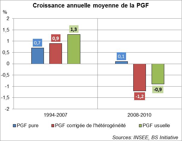
The usual CIF method overestimates the growth rate of potential GDP, while the pure CIF method offers a cautious but less pessimistic approach than the CIF method corrected for heterogeneity.

In terms of year-on-year rates and during periods of economic growth (1994-2007 in the chart below), the pure TFP method underestimates potential GDP less, and therefore requires greater fiscal consolidation efforts.

During periods of economic contraction (2008-2010 in the graph below), the pure PGF method underestimates the reduction in potential GDP less, resulting in a smaller fiscal consolidation effort.

While normative analysis would suggest choosing an estimation method based on the phase of economic activity in order to avoid underestimating the necessary fiscal consolidation effort, positive analysis leads us to consider that the pure PGF method would be appropriate during periods of growth but more questionable during periods of economic contraction.

The debate would then focus on the importance of the fiscal multiplier in a period of economic contraction: should public spending be increased in order to return to a path of sustainable potential GDP growth—which would justify moving away from the choice between pure PGF and conventional PGF?

Beyond the choice of modeling type, the assumptions used to integrate changes in production factors into the model require methodological choices that reveal a high sensitivity of the results to the assumptions defined.

Two examples are particularly noteworthy. The first concerns GDP in the non-market sector, which is considered exogenous in the French government’s model but endogenous in the European Commission’s model. A second example concerns the estimation of structural unemployment used to assess the PGF, specifically for one of its three determinants: labor. The European Commission estimates structural unemployment according to a Phillips curve (real wages fall as the unemployment rate rises), while the French government uses a wage bargaining model that includes certain fiscal variables.

All of these assumptions therefore require a methodological choice for their estimation. The labor factor will require significant forecasts in terms of net migration (the difference between the number of people entering the territory and the number of people leaving the same territory during a year), the activity rate, the growth of the working population, and the labor supply. The capital factor is estimated based on forecasts related to investment, renewable and non-renewable capacity utilization rates, refinancing costs, and depreciation rates used for productive investments. These components are themselves sensitive to economic reforms and require estimates of the success of the policies implemented and their implementation timeframes. These conditions are all the more important when it comes to anticipating the cyclical public balance, which depends on the effectiveness of a country’s fiscal policy, as will be discussed below.

2 – The impact of the estimate of potential GDP on the calculation of the structural balance

In simple terms, the structural balance can be broken down as follows:

Change in the structural balance as a percentage of potential GDP = Change in the actual balance as a percentage of actual GDP – Cyclical change in the public balance

The actual balance is therefore the sum of the cyclical balance and the structural balance, to which temporary budgetary measures may be added.

Potential GDP is therefore essential in this calculation as a component of the output gap (actual GDP-potential GDP). The structural balance is thus the sum of revenues (income tax, corporate tax, social security contributions, other compulsory levies) adjusted for expenditures (unemployment benefits, other benefits). Each revenue or expenditure item is weighted according to its contribution to total revenue/expenditure and its sensitivity to the output gap.

In short, an inaccurate estimate of potential GDP distorts the measurement of the sensitivity of each revenue/expenditure item to the output gap and therefore the level of variation in the structural balance as a percentage of potential GDP, and ultimately the necessary structural fiscal consolidation effort.

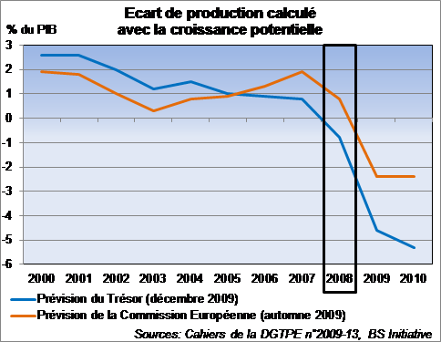
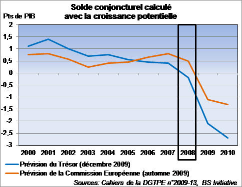
We can thus observe, with the European Commission or the Treasury, significant differences in forecasts for the output gap or the cyclical balance as a percentage of potential GDP. According to No. 2009-13 of the Cahiers de la DGTPE: as the forecasts for potential growth differ, the output gap implies a negative cyclical balance for the DGTPE in 2008 but a positive one for the European Commission (see graphs below).

These data allow us to observe the differences in estimates of potential GDP. To show the direct effect of the level of potential GDP on the level of fiscal consolidation required, we must take into account the calculation of the structural effort, which is the component of the change in the structural balance attributable to discretionary factors.

3 – Implication of potential GDP in determining the level of fiscal consolidation required

The structural effort directly determines the level of fiscal consolidation required for a given level of potential output. Determining this requires breaking down the change in the structural balance into the change in structural revenues and the change in structural expenditures.

The change in structural revenue as a percentage of potential GDP is the sum of three terms (the first discretionary, the next two non-discretionary):

– The ratio of new compulsory levies to potential GDP;

– The change in the ratio of non-compulsory revenue to potential GDP;

– The contribution of different elasticities to the variation in structural revenues.

The change in structural expenditure in terms of potential GDP points is the difference between two discretionary terms:

– The ratio between public expenditure in year n-1 and potential GDP in year n-1, weighted by the nominal growth rate of public expenditure adjusted for the growth rate of potential GDP;

– The product of the elasticity of unemployment expenditure to the output gap, the share of expenditure related to unemployment benefits in total expenditure, and the variation in the output gap.

The structural effort corresponds to all discretionary terms, i.e.:

– The ratio of new compulsory levies to potential GDP;

– The ratio of public expenditure in year n-1 to potential GDP in year n-1, weighted by the nominal growth rate of public expenditure adjusted for the growth rate of potential GDP;

– The product of the elasticity of unemployment expenditure to the output gap, the share of expenditure related to unemployment benefits in total expenditure, and the change in the output gap.

Conclusion

Estimating potential GDP requires important methodological choices that determine the assessment of the structural budget balance and , ultimately, the level of fiscal consolidation required.

A key debate concerns the appropriate methods for assessing potential GDP given a given phase of economic activity. In periods of economic contraction, structural budget balance targets may be postponed due to the effect of the fiscal multiplier, the estimation of which is also a matter of debate. It was precisely these two debates that led the European Commission, in May 2013, to grant France two additional years to achieve a budget deficit of less than or equal to 3%.

Reference:

– Dominique Ladiray, Gian Luigi Mazzi, Fabio Sartori: « Statistical Methodsfor Potential Output Estimation and Cycle Extraction, » European Commission, 2003.

– « Growth and public finances, » The French Economy 2004-2005.

– Laurence Boone: “Potential GDP: the consequences of singing too loudly with the Cassandras,” Les Echos, July 20, 2009.

– European Commission: “Assessment of France’s National Reform Program and Stability Program 2013,” page 39, May 29, 2013.

– Christophe Cahn, Arthur Saint-Guilhem: « Potential growth: where do the differences between some major developed economies come from? » , Bulletin de la Banque de France, No. 155, November 2006.

– Pierres-Yves Cabannes, Alexis Montaut, Pierre-Alain Pionnier: « Evaluating total factor productivity: the contribution of measuring the quality of capital and labor, » INSEE, The French Economy, 2013 edition.

– Thibault Guyon, Stéphane Sorbe: « Structural balance and structural effort: towards a breakdown by sub-sector of public administrations, » Directorate General of the Treasury and Economic Policy, No. 2009/13, December 2009.